Pearson's Correlation

This guide delves into the meaning and computation of Pearson's correlation coefficient. It begins with generating two sample datasets, and then walks through the steps (and intuition) for measuring their correlation. It's breif and to the point -- all necessary code is provided.

We'll start by generating a sample dataset based on the Sinusoid line and a random dataset, both of equal length:

import numpy as np

tab1 = np.sin(0.3 * np.arange(0, 2 * np.pi, .001))
tab2 = np.random.random(len(tab1))

Let's visualize them:

import matplotlib.pyplot as plt

plt.plot(tab1); plt.title("tab1"); plt.show()
plt.plot(tab2); plt.title("tab2"); plt.show()

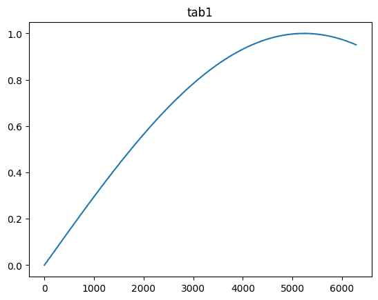
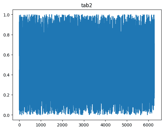
Since we're comparing the Sin(0.3x) curve with random data, the correlation should be very low (~0).

Now, let's use a prebuilt function of numpy to calculate the coefficient, and then see if we can arrive at that value on our own. We will also introduce the notion of understanding our data as vectors in hyperdimensional space.

The following code ensures that both data sets are of equal length, which is a prerequisite for Pearson's correlation, and uses numpy's corrcoef function to calculate it. The output will be between -1 and 1, with proximity to 0 indicating non-correlation.

# Ensure both data sets are equal length
print("Dimensions in data:", len(tab1), len(tab2))

# Calculate correlation with numpy's corrcoef function
correlation = np.corrcoef(tab1, tab2)[0, 1]
correlation

Output:

    Dimensions in data: 6284 6284
    
    -0.006317307879290855

Looks good. The datasets have an equal number of points and the corrcoef function gave us a value near 0 -- indicating, as expected, a lack of meaningful correlation. Now, let's go behind the scenes and step through the process. What does Pearson's correlation coefficient represent, and how is it determined?

We'll split it into three basic steps / components:

1. The first step is to understand that any dataset can be formulated as a vector - a single point in n-dimensional space with magnitude and direction. The "n" dimensions correspond to the number of data points, with each getting its own dimension. The vector's projection onto a specific axis (or dimension) i yeilds the i th point of the dataset, and so on. What results is a vector, pointing to a specific coordinate in hyperdimensional space which is determined by every entity (x0, x1, x2, ... xn) in the dataset.

2. In order to measure the datasets' correlation, we should rule out / ignore some commonality. When comparing salaries or house prices, for example, the fact that they are positive values is not important and therefore shouldn't be considered for correlation. This is acheived by measuring the datasets' standard deviations, rather than the original data. Standard deviation is the distance, or difference, of each datapoint from the overall average of the whole dataset. By subtracting the average, the dataset is normalized -- it no longer makes a difference where the dataset lied on the y-axis.

3. Both datasets are of equal length -- they have the same number of dimensions. Therefore, it is straightforward to compare them as vectors. When doing so, we will purposefully ignore the magnitude of the vectors. The magnitude represents each datasets' scale, which should not affect their correlation. Instead, we want to identify the shared trend (if any) between the datasets. Do they increase or decrease together? And if so, by how much? This what Pearson's correlation coefficient measures. The angle between the vectors, or more specifically -- the angle's cosine -- yeilds Pearson's correlation coefficient.

The code:

# Step 1: Define each dataset as an n-dimensional vector. Check to ensure their dimensionality is equal.
print("Dimensions in data:", len(tab1), len(tab2))

# Step 2: Mean-center the datasets.
tab1_centered = tab1 - np.mean(tab1)
tab2_centered = tab2 - np.mean(tab2)

# Step 3: Determine the cosin of the angle between the normed vectors
cosin_theta = np.dot(tab1_centered, tab2_centered) / (np.linalg.norm(tab1_centered) * np.linalg.norm(tab2_centered))

cosin_theta

Output:

Dimensions in data: 6284 6284

-0.006317307879290849

Now, let's check if our calculation yeilds the same value as the built-in operation:

abs(correlation - cosin_theta) < 1e-16

Output:

True